The Machines · Statistics & machine learning

neural

Feed-Forward Neural Networks — machines/neural.shoddy

Summary

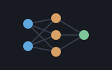
neural gives Shoddy the classic small neural network — a program that learns a pattern from examples by adjusting stored numbers called weights. This one has one hidden layer, a middle rank of Tanh units between input and output. It is small enough to hold entirely in your head. It trains by mini-batch stochastic gradient descent: take a small shuffled batch of examples, measure the error, and nudge every weight a little downhill. A Net is a plain record of four fields: two weight matrices and two bias vectors. The design's one big win is that a gradient has the same shape as the network. A gradient is the set of nudges, one per weight, so the very same record represents both. Accumulating, averaging, and applying an update all fall out of two words — NetAdd and NetScale. No zeroing loops, no mutable scratch arrays: training is a pure Fold over epochs (full passes through the data), and each epoch is a Fold over shuffled mini-batches. The same identity carries momentum, because a velocity is a Net too.

It does two jobs, chosen by a head. Regress reads the output layer as-is and fits squared error — predict a number, score it on how close. Classify reads it through Softmax, which turns raw scores into probabilities that sum to 1, and fits cross-entropy — predict a category, score it on how often it's right, and get a probability for every candidate. Those look like different networks in most textbooks. Here they share one backward pass, for a reason worth knowing (see Under the Hood).

A Brief History of Backpropagation

The idea of a network of simple threshold units goes back to McCulloch and Pitts in 1943. Rosenblatt's perceptron of 1958 could even learn — but only a single layer of it. Minsky and Papert's 1969 book Perceptrons proved crisply how little a single layer can do. What was missing for the next fifteen years was not the idea of hidden layers but a way to train them: if the output is wrong, how much of the blame belongs to a weight buried two layers deep? The answer is to apply the chain rule — the calculus rule for tracing a change through nested steps — sweeping the error backwards through the same connections the signal came forward through. That answer was found several times: by Werbos in 1974, and famously by Rumelhart, Hinton, and Williams in 1986, who named it backpropagation and showed the world it worked. Every modern deep-learning framework, however vast, is still doing exactly this. A forward pass remembers its activations — each unit's computed output. A backward pass turns one subtraction at the output into a gradient for every weight. The weights then take a small step downhill. This machine implements that 1986 algorithm at its original scale, where you can watch every part of it happen.

Why It's Useful

Sometimes the relationship you want to learn from data isn't a line, and no amount of squinting at stats' LinFit will make it one. A one-hidden-layer network is the smallest honest tool for that job. Given enough hidden neurons it can approximate any reasonable function. With a few hundred rows and a few thousand epochs, it does so on classroom hardware in classroom time. Reach for neural when you have a table of numeric inputs and either a numeric target whose mapping bends, or a label drawn from a short fixed list. It builds on matrix: the forward pass is a MatVec, and the weight gradients are Outer products. It also uses random (each epoch shuffles), file (weights save and load as plain text), and recio (the binary model format underneath NetSaveBin/NetLoadBin).

User's Guide

Build a net, train it, ask it questions. The training data is a List of input rows (each an Array Of Number) and a List of target numbers.

Include "neural.shoddy"

Def Main()
    Seed(0)                                  ' reproducible runs — do this first
    Let xs = { ToArray({ 0.1 }), ToArray({ 0.5 }), ToArray({ 0.9 }) }
    Let ys = { 1.2, 2, 2.8 }                 ' y = 2x + 1

    Let n0 = NetNew(1, 4, 1)                 ' 1 input, 4 hidden, 1 output
    Let n = NetTrain(n0, xs, ys, 0.1, 3, 500, [ Drop Drop ])   ' silent report

    Print(NetOut(n, ToArray({ 0.7 })))       ' close to 2.4
    NetSave("wts.txt", n)
    Let m = NetLoad("wts.txt", 1, 4, 1)      ' same predictions to ~1e-10

Classification is the same machine wearing the other head. Targets become one-hot vectors — all zeros, with a single 1 marking the class — instead of numbers. The hyperparameters (the training settings: rate, momentum, batch, epochs) travel as a Plan, and the answer comes back as a probability for each class:

Include "neural.shoddy"

Def Main()
    Seed(0)
    Let raw = { ToArray({ 5.1, 3.5 }), ToArray({ 6.7, 3.0 }), ToArray({ 5.0, 3.4 }) }
    Let ys  = { NetOneHot(1, 2), NetOneHot(2, 2), NetOneHot(1, 2) }   ' 2 classes

    Rem centre and scale the inputs, and keep the scaler — you will need
    Rem exactly this transformation again at prediction time
    Let sc = ScalerFit(raw)
    Let xs = Map(raw, Fn(x) => ScalerApply(sc, x))

    Rem ClassPlan(rate, momentum, batch, epochs)
    Let n = NetFit(NetNewScaled(2, 6, 2), ClassPlan(0.1, 0.9, 3, 300), xs, ys, [ Drop Drop ])
    Print(NetClassAccuracy(n, xs, ys))       ' 1
    Print(NetPredict(n, Classify(), First(xs)))   ' probabilities, summing to 1

    Rem save weights + head + scaler as one artifact, then predict from RAW input
    ModelSave("model.bin", Model(n, Classify(), sc))
    Let m = ModelLoad("model.bin")
    Print(ModelClassOf(m, ToArray({ 5.1, 3.5 })))    ' 1 — no scaling by hand

A few things worth remembering:

• Seed first if you want the same run twice. NetNew and NetTrain's shuffle are the machine's only impure words. One Seed(k) at the top of Main pins them both.
• The report quotation runs after every epoch — you decide when to print and when to pay for metrics. [ Drop Drop ] is the silent report. The pattern If epoch Mod freq = 0 Then ... prints every freq-th epoch and costs nothing in between.
• Batches tile the whole epoch. Each epoch shuffles the row indices and takes Floor(n / batSize) consecutive chunks. The remainder rows (fewer than a full batch) are dropped that epoch — a different remainder each time, since the shuffle is fresh.
• Scale your data — and keep the scaler. Tanh neurons saturate: fed inputs far from zero, their output flattens and learning stalls. Inputs somewhere near [-1, 1] keep the gradients alive. You can do it by hand (divide ages by 100, incomes by 100 000) or let ScalerFit centre each column on its mean and divide by its spread. Either way, the prediction side must apply the identical transformation. That is why Model stores the scaler beside the weights and ModelPredict takes raw inputs. Rebuilding the transformation by hand in a second program is the classic way to end up serving a model inputs it was never fitted on, with nothing to warn you.
• Momentum is usually worth switching on. NetFit's Plan carries a momentum coefficient. 0.9 is the conventional starting point, and it typically reaches a given loss in a fraction of the epochs plain descent needs. Setting it to 0 reduces NetFit to exactly the descent NetTrain performs — bit for bit, which the machine's tests assert.
• Fit the scaler on the training rows only. Letting the held-out rows influence the centring leaks them into training and quietly flatters the test score.
• Two serialization formats, one canonical order. Serialization means writing a value out, as text or bytes, so it can be loaded back later. NetSave writes text, one number per line, in the traditional order: input-hidden weights input-major, hidden biases, hidden-output weights hidden-major, output biases. Weight files therefore interchange with the classic C# demo (Str writes 10 significant digits, so a text round trip reproduces predictions to about 1e-10 relative). NetSaveBin writes the same sequence as raw 8-byte doubles behind a self-describing header. So NetLoadBin(path) needs no architecture arguments, and the round trip is bit-exact.

The mills use this machine end to end, and reading iris and demographics side by side is the fastest way to see the difference between the heads. iris predicts a category (species) with the Classify head. It is scored on how often it is right, and it reports how sure it was. demographics predicts a number (income) with Regress and is scored on how close it gets. Both split the same way: a trainer that writes a model file, and a predictor that reads one. iris trains in about four seconds, which makes it the one to run when changing this machine.

Under the Hood: Gradients With the Net's Shape

You don't need any of this to use the machine — it's here for the curious.

A Net holds W1 (hidden×input), B1, W2 (output×hidden), and B2. The forward pass is two lines of matrix algebra: h = Map(VAdd(MatVec(W1, x), B1), Tanh), then o = VAdd(MatVec(W2, h), B2). NetEvalAt returns both h and o in a NetEval record, because the backward pass needs the hidden activations it just computed.

The backward pass is four lines. For one example with target y: the output signal is o - y. The hidden signal carries that back through W2 transposed, then multiplies by the tanh derivative, written (1 - h)(1 + h) from the activations themselves. Each weight matrix's gradient is the Outer product of its layer's signal with its layer's input. The result is assembled straight into a Net — gradient and network, same shape.

Both heads share that pass, and the reason is a small piece of calculus worth carrying around. Differentiate squared error through an identity output, and the error signal arriving at the output pre-activation is output - target. Differentiate cross-entropy through a softmax output, and it is probabilities - target. The exponentials and the logarithm cancel exactly, and what is left is the same subtraction. So NetGradAt has precisely one line that knows which head it is working for — oSig, where the head decides how to read the output layer. Every other line of the backward pass, every weight gradient, the mini-batch averaging, the momentum, and the serialization are shared verbatim. Regression's NetGrad is a one-line wrapper over it rather than a second copy, so the two cannot drift apart. This is asserted, not assumed: the machine's tests difference both losses numerically against the analytic gradient, every parameter, and swapping one head for the other makes them fail.

That shape-sharing is the whole design. A mini-batch step is Fold-ing NetAdd over the per-example gradients, one NetScale by 1/batchsize to average, and one more NetScale by -lr plus a final NetAdd to descend. The classic imperative version zeroes four accumulator arrays and runs ten nested loop blocks. The algebra here has no accumulators at all — purity made the bookkeeping vanish. The Tanh activation itself is a runtime builtin (it needs native precision and saturates safely at ±1). That is the same division of labor the whole library follows: the runtime supplies the primitives, Shoddy derives the rest.

Word Reference

Every word, plus the Net, NetEval, Head, Plan, Scaler and Model types

The types

Building and combining the constructors are impure: Rnd

Running the network

Training NetTrain and NetFit shuffle: impure

Measuring

Scaling the inputs

Saving and loading effectful; call from Main

Who Uses It

	User	How
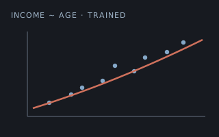	demographics	The 8-100-1 regression — mini-batch SGD with momentum and the binary save/load pair.
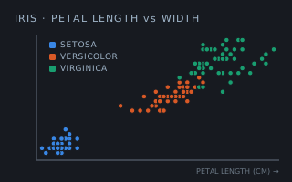	iris	The 4-8-3 classifier — softmax and cross-entropy, the input Scaler, and the saved model the predictor reloads.

The Machines It Uses

	Machine	Why
	file	ReadLines / WriteLines carry the text model format.
	matrix	The algebra under every forward and backward pass — MatVec, Outer, Transp and the vector arithmetic.
	random	Shuffle deals the mini-batches; RandomRange scatters the initial weights.
	recio	GetRec / PutRec are the binary model file — the bit-exact save/load contract.
	seq	ZipWith walks a layer's weights against its inputs.