simplex

Linear Programming — machines/simplex.shoddy

Summary

simplex solves the kind of problem where you're trying to do something as cheaply as possible while still meeting a list of hard requirements. You hand it three things:

a list of costs — how much each ingredient adds to the bill
a grid of numbers saying how much each ingredient contributes to each requirement
the requirements themselves — you must end up with at least this much of each

It hands back the cheapest mix that satisfies every requirement — the exact amounts to use, the total cost, and a little extra bookkeeping that tells you how sensitive that answer is to the numbers you gave it. Under the covers it runs the simplex method, the seventy-year-old workhorse algorithm for exactly this shape of problem. It is built on the sparse machine for the constraints and the matrix machine for the small dense square at the heart of it.

Two doors, one solver. Optimize takes a Problem with an ordinary dense Matrix and is the one to learn first. SpOptimize takes an SpProblem holding the same constraints in sparse form, for the big thin problems where writing every zero down would be the expensive part. They are not two implementations: Optimize converts and calls SpOptimize, so both walk the same pivots and answer the same numbers. Integer answers are mip, one floor up.

A Brief History of Linear Programming

The story starts in 1947 with an American mathematician named George Dantzig. He was working for the U.S. Air Force on the dreary-sounding but genuinely enormous problem of planning — how to schedule the training, supply, and deployment of an entire military without wasting men, money, or materiel. Problems like that have thousands of interlocking choices and thousands of constraints. Until then there was no general way to find the best answer rather than merely a workable one. Dantzig framed the whole thing as what we now call a linear program: a linear cost to minimise, and a wall of linear inequalities to respect. Then he invented a method to actually solve it, and called it the simplex method.

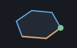
The geometric picture is lovely, and worth carrying in your head. Every constraint is a flat wall. Together, all the walls enclose a shape — a many-sided crystal called a polytope — and every point inside that shape is an allowed answer, a menu that breaks none of the rules. The magic fact Dantzig leaned on is that the very best answer is never floating somewhere in the middle. It always sits at a corner of that crystal, where several walls meet. So instead of searching the whole interior, the simplex method just visits corners. It starts at one corner, looks along each edge leading away from it, and walks to whichever neighbouring corner improves the cost the most. It keeps stepping from corner to better corner along the edges of the polytope until no neighbour is any better. Then, by that same magic fact, it's standing on the answer.

It worked, and it kept working, on problems far larger than anyone in 1947 would have believed. The simplex method is routinely named one of the most important algorithms of the twentieth century. It quietly underpins logistics, manufacturing, finance, and airline scheduling to this day. The theory grew up around it too. The Soviet mathematician Leonid Kantorovich had reached related ideas independently in 1939. Much later, in 1984, Narendra Karmarkar found a rival family of methods that cut through the interior of the polytope rather than walking its corners. But the corner-walking simplex method never retired. It remains one of the two algorithms every serious solver still ships. This machine implements it in a few hundred lines of Shoddy — no punch cards, no Pentagon.

Why It's Useful

An enormous number of real decisions have the same shape: you have some knobs you can turn, each knob costs something, and turning them affects a handful of things that all have to come out right. A cafeteria wants the cheapest menu that still hits everyone's calorie and protein targets. A refinery wants the most profitable blend of crude oils that still meets the octane spec. A delivery company wants to move goods between warehouses for the least fuel while still getting enough to each shop. Written down, these are all the same puzzle — minimise a cost, subject to a set of "at least this much" constraints, with nothing allowed to go negative — and that puzzle is called a linear program. It's one of the most solved problems in all of computing precisely because it turns up everywhere. Reach for simplex whenever you can phrase your question as "what's the cheapest way to satisfy all of these at once?" The relationships between your knobs and your requirements must be straight-line ones (double an ingredient, double its contribution). If your problem also lives in a file, the mps machine reads the standard file format for these problems and hands you exactly the value this machine expects.

User's Guide

You describe a problem with three pieces, and they must line up. The Costs are one number per variable — what a unit of each variable adds to the total you're minimising. A is a matrix with one row per requirement and one column per variable, saying how much each variable contributes to that requirement. Rhs ("right-hand side") is one number per requirement — the amount you must reach. The machine reads every constraint as A x >= Rhs (at least this much), with every variable held at zero or above.

Include "simplex.shoddy"

Def Main()
    ' Cheapest mix of two foods that meets two nutrient targets.
    ' minimize 4*meat + 2*bean
    '   meat + bean >= 10     (bulk)
    ' 3*meat + bean >= 18     (protein)
    Let costs = { 4, 2 }
    Let a     = MatFromRows({ { 1, 1 }, { 3, 1 } })
    Let rhs   = { 10, 18 }

    Let sol = Optimize(Problem(costs, a, rhs))

    Print(Status(sol))                       ' OPTIMAL
    Print("cost " & Str(Cost(sol)))          ' cost 28
    Each(X(sol), Fn(v) => Print(Str(v)))     ' 4 then 6  (meat, bean)
    Each(DualPrices(sol), Fn(v) => Print(Str(v)))  ' 1 then 1 (shadow prices)

The answer says: use 4 of the first food and 6 of the second, for a total cost of 28, and there's no cheaper way to hit both targets. A few things worth remembering:

Everything is "at least." Constraints are always read as A x >= Rhs. If your real requirement is an upper limit ("no more than 18"), negate that row and its right-hand side to flip it around. If it's an exact equality, supply it as two rows — one >= and one <= of the same thing. The mps machine does exactly this bookkeeping for you when it reads a file, so you rarely have to do it by hand.
Variables never go negative. Every variable is held at zero or above automatically — you don't add those constraints yourself. That's the standard convention for linear programs, and it's baked in.
Always check the Status first. A healthy answer comes back "OPTIMAL". But not every problem has a good answer. If your requirements contradict each other so that no mix can satisfy them all, you'll get "INFEASIBLE". If the problem is malformed in a way that lets cost run off to nothing, you'll get "UNBOUNDED-OR-INFEASIBLE". And in the very rare case a problem is so large or awkward that the search doesn't settle, you'll get "MAXITER". In all those cases the X, Cost, and the rest are empty or meaningless — the status is telling you not to trust them.
The extra numbers are worth reading. Alongside the answer you get DualPrices — one shadow price per requirement, telling you how much the total cost would move if you nudged that requirement up by one unit. In the example, both prices are 1, meaning each extra unit of either target would cost you one more. That's the "sensitivity analysis" managers pay real money for: it tells you which constraint is really pinching. Reduced does the mirror-image thing per variable, and Iterations reports how many corners the method had to walk.
For a big problem, come in the sparse door. If your constraint grid is large and mostly zeros — which is what a real problem read out of a file usually is — build an SpProblem and call SpOptimize. It is the same solver and the same answer, with the zeros never written down. The mps machine's LoadMpsSp hands you one directly.

Under the Hood: Walking the Corners

You don't need any of this to use the machine — it's here for the curious, and for anyone who has met the simplex method before and wants to know which variant this is.

It's the revised simplex method, and it solves the dual. The plain simplex method keeps a big rectangular tableau and pivots on it. The revised method — what this machine uses — keeps only the small square that matters: the inverse of the current basis (the set of variables currently in play), a matrix called binv. Rather than rewrite a whole table each step, it updates that one inverse with an eta-style row operation (UpdateBinv), which is the same pivot in cheaper clothing. And rather than attack your problem head-on, it solves its dual: the mirror-image problem max Rhs.y subject to Transp(A) y <= Costs. This isn't a detour — it's a shortcut. At the optimum of that dual, the simplex multipliers turn out to be exactly the primal answer x you were after, so one solve gives you both sides at once.

Each step is a price, a pick, and a pivot. The loop (Solve) prices out every non-basic variable to find the one with the most positive reduced cost — the steepest downhill edge — in PickEnter. That's the corner-to-corner walk from the history section, made arithmetic. Then PickLeave runs the ratio test: as the entering variable grows, it finds which basic variable hits zero first, and that's the one that leaves. Swap the two, update the basis inverse, and step to the next corner. When no variable has a positive reduced cost, there's no downhill edge left: you're on the answer, and the loop reads the optimal basis back out.

Pricing is where the sparsity pays, and it pays exactly. Pricing is the bulk of the work — it visits every column on every step — and in a real problem most of what it visits is zeros. So the dual matrix is a Sparse: its slack and artificial columns are single stored numbers rather than a materialised identity, and SpColDot multiplies only what is actually there. The same goes for FTran, which forms the step direction by reaching into just the rows the entering column occupies. This changes no answer, and that is not a hope but a property: a term that was zero contributed nothing to the sum, so leaving it out moves not one bit of the result. The pivots, the iteration count, and the last decimal place are all what they were when every zero was written down and read back.

Getting a feasible start with big-M. The simplex method has to begin standing on some valid corner, and finding one isn't always free. If every cost is zero or positive, the obvious slack start is already valid and the machine uses it directly — no fuss, exactly the classic textbook run. But a negative cost makes the dual's slack start infeasible. So for each such variable the machine negates that row and adds an artificial variable with a huge penalty coefficient (bigM, scaled to your data). The penalty is so steep that the method is driven to push every artificial back down to zero on its way to the optimum. If it manages that, the artificials vanish and the answer is honest. If one stubbornly refuses to leave, that's the tell-tale of a problem with no real solution, and you get "UNBOUNDED-OR-INFEASIBLE" rather than a confident lie.

Reading the answer back. At the optimum the dual's structural variables (the first m of them, one per requirement) are the primal constraints' shadow prices — that's DualPrices. Its slack variables (the next n, one per variable) are the primal variables' reduced costs — that's Reduced. The primal answer X itself is read from the simplex multipliers, with the sign flips from the big-M start undone. Everything is pure: Optimize reads its Problem, does its arithmetic, and hands back a Solution, touching nothing outside itself. Shoddy by name — but the algorithm inside is the real thing.

How big is too big. The basis inverse is kept whole and dense, and it is n×n where n is the number of variables — not constraints. Every pivot rewrites all of it, so that square is the ceiling: this is a solver for problems with hundreds of variables, and it does not mind how many constraints they have. (Constraints are cheap now in a way they were not: each is one sparse column in the dual.) Past that, the answer the field reached long ago is to stop keeping the inverse whole — the product form of the inverse, or a sparse LU with the update mathematics that goes with it. Both are real machinery and neither is here. They would fit behind these same two words if the day came.

Word Reference

Every word, plus the Problem, SpProblem and Solution types

The types

Word	Description
Problem(Costs, A, Rhs)	A linear program to solve. `Costs` is an array of numbers, one per variable, to be minimised. `A` is a Matrix with one row per constraint and one column per variable. `Rhs` is an array of numbers, one per constraint. The problem is read as: minimise `Costs . x` subject to `A x >= Rhs` and `x >= 0`.
SpProblem(Costs, SA, Rhs)	The same statement of the same problem, with `SA` a Sparse instead of a dense `Matrix`. What to build when the grid is large and mostly zeros; mps and mip both speak this one.
Solution(Status, X, Cost, DualPrices, Reduced, Iterations)	What `Optimize` hands back. `Status` is a string (`"OPTIMAL"`, `"INFEASIBLE"`, `"UNBOUNDED-OR-INFEASIBLE"`, or `"MAXITER"`). `X` is the array of optimal variable values; `Cost` its total cost. `DualPrices` is the shadow price per constraint (how much `Cost` moves per unit of that `Rhs` — the sensitivity analysis); `Reduced` the reduced cost per variable; `Iterations` the number of simplex steps taken. When `Status` isn't `"OPTIMAL"`, the numeric fields are empty or meaningless.

Solving

Word	Description
Optimize(p)	Solves the `Problem` `p` and returns a `Solution`. Pure, with no side effects. Always check `Status` before trusting the rest. Internally it converts `A` to sparse and calls `SpOptimize`, so it is the same walk to the same answer.
SpOptimize(p)	The same, for an `SpProblem` — the solver proper, and the one to call when the problem is big enough that building a dense `Matrix` first would be the expensive part. Refuses a problem whose matrix does not match the length of its costs and its right-hand side.

Those two are the whole public surface. Everything else in the file — the pricing scan, the ratio test, the basis-inverse update, the dual construction — is internal plumbing, described above for the curious rather than offered as words to call.

Who Uses It

	User	How
	mip	Every node of its search is an `SpOptimize`, and the `Solution` that comes back decides whether to branch, prune, or keep the answer.
	mps	Builds its output to fit — `LoadMpsModel` returns exactly the problem `Optimize` consumes, and `LoadMpsSp` the one `SpOptimize` does.
	simplex-from-mps	`Optimize` solves what the MPS file describes; the report prints its status, objective and sensitivity numbers.

The Machines It Uses

	Machine	Why
	matrix	The basis inverse is a dense matrix — `Ident`, `MatFromRows`, `MatGet`, `Dot` — as is the `A` a `Problem` states.
	sparse	The constraint matrix the solver actually walks — `SpColDot` prices a column, `SpTransp` turns the primal round once to build the dual, and `SpFromMat` is how a dense `Problem` gets in.